Same result, 3 seconds or 30 minutes. Query optimization in Databricks
Seven techniques that decide whether the engine does a little work or a lot
Two engineers were asked the same question. Which products earned the most revenue last month?
Both wrote SQL. Both got the same numbers, down to the cent.
The first query returned in three seconds. The second scanned billions of rows, moved a few hundred gigabytes across the network, held a large cluster busy, and finished in thirty minutes.
Nobody reviewed the second query, because it was correct. That is the quiet trap. Correctness is easy to see. Cost is not.
The difference between three seconds and thirty minutes was never the result. It was the execution.
Your SQL is a request, not an instruction
It helps to know what happens between the moment you press run and the moment the answer appears.
First the parser checks the syntax and resolves your table and column names. Then the engine builds a logical plan, which is a description of what you asked for: scan these tables, apply this filter, join on this key, group by this column.
Then the optimizer rewrites it. Using rules, table statistics, and what it knows about the cluster, it produces a physical plan: the actual sequence of scans, shuffles, sorts and joins the workers will run.
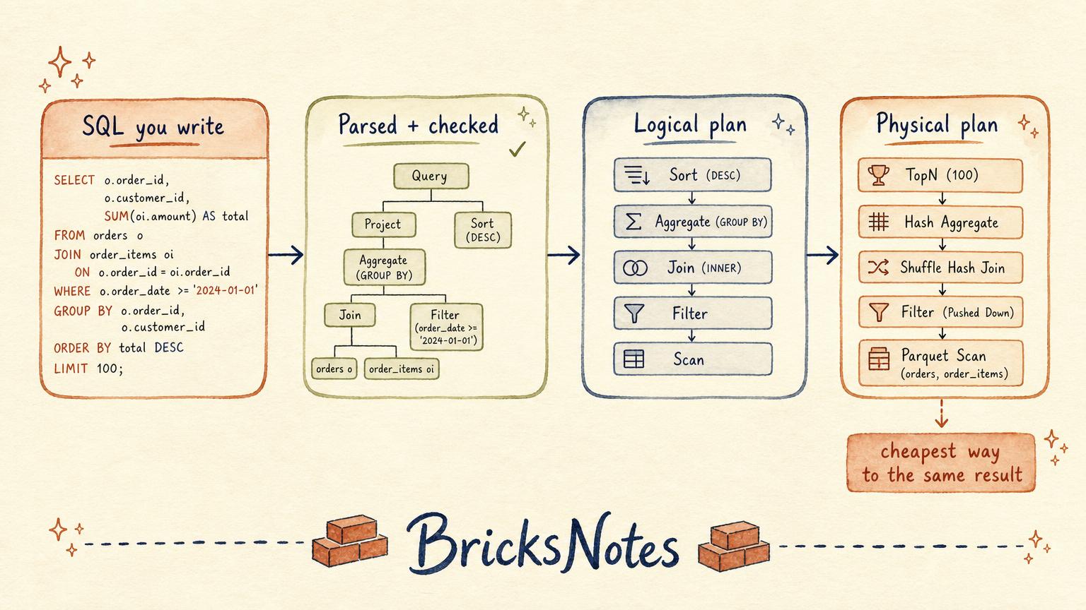
The important thing is what the optimizer is asking itself. It is not asking "is this query correct?" It assumes you got that part right.
It is asking one question:
What is the cheapest way to produce the same result?
Every optimization technique below is a way of helping it answer that question well. We walk through the same journey with runnable examples in the Spark SQL lesson, and the plan reading habits in the Debugging and Monitoring lesson.
https://youtu.be/2vg3Z41HtUY
1. Predicate pushdown: filter at the storage layer
A predicate is a filter. Pushdown means the filter is applied as early as possible, ideally while the files are being read rather than after.
Without pushdown, the engine reads three years of data into memory, then throws away everything except last month. With pushdown, the file reader skips files whose statistics say they cannot contain last month at all.
-- the filter can be pushed into the scan
SELECT product_id, SUM(amount) AS revenue
FROM sales
WHERE sale_date >= '2026-07-01'
  AND sale_date <  '2026-08-01'
GROUP BY product_id
Two habits keep pushdown working.
Filter on the raw column, not on a transformed version of it. WHERE YEAR(sale_date) = 2026 hides the column inside a function, and the reader can no longer compare it against file statistics. Write a plain range instead.
Filter before joining, not after. A filter applied after a join has already paid for the join.
Delta tables make this stronger, because every file carries min and max values per column in the transaction log. That is why file layout matters so much, and why we cover it in the Delta Lake lesson.
2. Column pruning: stop reading what you never use
Parquet and Delta store data by column, not by row. That means the engine can read three columns out of eighty and never touch the rest.
SELECT * throws that advantage away.
-- reads 3 columns
SELECT order_id, customer_id, amount FROM orders

-- reads all 80
SELECT * FROM orders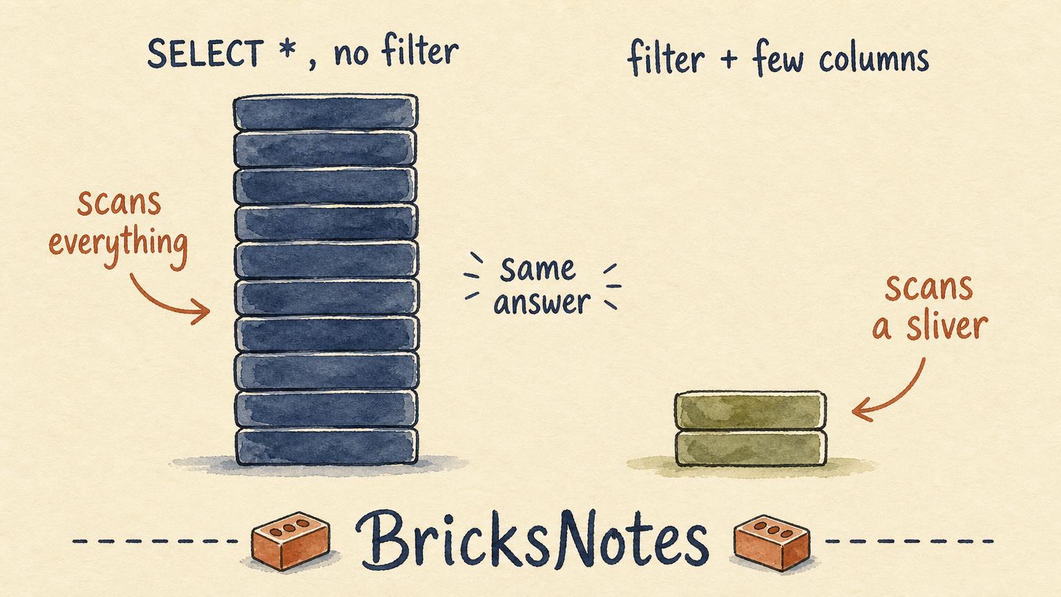
This sounds too simple to matter. On a wide table it is often the single largest saving available, and it costs nothing but discipline. It also makes shuffles cheaper later, because a shuffle moves whole rows. Twenty unused columns is twenty columns of network traffic per row.
The File Formats lesson shows why columnar storage behaves this way, and our article on CSV, JSON, Parquet and Delta compares what each format can and cannot skip.
3. Partition pruning: skip whole directories
If a table is partitioned by date, a filter on date lets the engine ignore entire partitions without opening a single file inside them.
This is the fastest form of skipping, and also the easiest to break.
-- prunes: engine compares the partition value directly
WHERE event_date = '2026-08-27'

-- often does not prune: the column is wrapped in a function
WHERE DATE_FORMAT(event_date, 'yyyy-MM-dd') = '2026-08-27'

-- does not prune: the filter is on a different column
WHERE event_timestamp >= '2026-08-27 00:00:00'
The failure is silent. The query still returns the right answer. It just reads everything.
A related trap is partitioning on a high cardinality column, which produces millions of tiny files and makes every read slow. On Databricks the modern answer is usually liquid clustering rather than hand-picked partitions, which we compare in Z-ORDER or liquid clustering and teach in the Partitioning and Performance lesson.
4. Join strategy: move the small side, not the big one
A join is the moment your data has to physically move.
If both tables are large, the engine repartitions both by the join key and sends them across the network so matching rows land together. That is a shuffle join, and it is expensive but general.
If one side is small, the engine can send a full copy of it to every worker instead. Now the large table never moves. That is a broadcast join, and it is often an order of magnitude faster.
from pyspark.sql import functions as F

enriched = orders.join(F.broadcast(dim_customers), on="customer_id", how="left")
Databricks often makes this choice for you. It makes it well when it knows the small side is small, and it guesses when the small side is the output of a long chain of filters and aggregations. That is when stating the hint yourself pays off.
We go deeper in the join that ran for seven hours, and practise both styles in the Joins and Aggregations lesson.
5. Data skew: one worker doing everyone's work
You have seen this shape. The job reports 199 of 200 tasks complete within two minutes, then sits on the last one for forty minutes.
That is skew. The data was split by key, and one key holds far more rows than the rest. Usually it is something ordinary: a NULL customer id, a default value like unknown, a single enormous account, or one country that is most of your traffic.
Adaptive query execution can split some skewed partitions automatically. When it cannot, the usual fix is to separate the heavy key or spread it with a salt.
# handle the dominant key separately, then union the results
heavy = events.filter(F.col("customer_id") == "unknown")
rest  = events.filter(F.col("customer_id") != "unknown")
The full walkthrough is in one task ran for forty minutes.
6. Table statistics: the optimizer is only as good as what it knows
The optimizer decides between broadcast and shuffle, and between join orders, based on estimated row counts and column sizes. Those estimates come from statistics.
If statistics are missing or stale, the estimate can be wrong by orders of magnitude. A table the optimizer believes holds ten thousand rows might hold ninety million. It picks a broadcast, the broadcast does not fit, and the job either crawls or fails.
ANALYZE TABLE sales COMPUTE STATISTICS FOR ALL COLUMNSOn Databricks, predictive optimization handles most of this maintenance for managed tables. It is still worth knowing the mechanism, because when a plan looks irrational the first thing to check is what the optimizer believed.
7. Adaptive query execution: correcting the plan mid-flight
Some things cannot be known before the query starts. The real size of an intermediate result, for example.
Adaptive query execution lets the engine re-plan while running. After a stage completes, it looks at actual statistics and can switch a shuffle join to a broadcast join, merge many tiny partitions into a sensible number, or split a skewed partition.
It is enabled by default on Databricks, and it is a safety net rather than a strategy. It cannot undo a full table scan you asked for, and it cannot invent a partition filter you did not write.
Caching helps, and it also hides
Caching a dataset you read repeatedly in the same session is useful.
Caching to make a badly written query feel acceptable is not. The work is still happening, the memory is still occupied, and the underlying problem is now invisible until the data grows or the cache is evicted.
Cache deliberately, and only after the query itself is reasonable.
The habit that matters more than the seven techniques
Learn to read the execution plan.
In Databricks you can start with EXPLAIN FORMATTED, then use the Spark UI to compare what was estimated with what actually happened.
EXPLAIN FORMATTED
SELECT product_id, SUM(amount)
FROM sales
WHERE sale_date >= '2026-07-01'
GROUP BY product_id
Look for six things:
- Full table scans where you expected a filter
- Large shuffles, especially several in a row
- Expensive sorts that nothing asked for
SortMergeJoinwhere aBroadcastHashJoinwas possible- Missing partition or file filters in the scan node
- Estimated row counts that are far from the actual row counts
That last one is the most useful signal on the page. When estimates and reality diverge badly, the plan was chosen for a query that does not exist, and everything downstream is built on that mistake.
A query that runs is not automatically a good query
Success is not a performance metric. Before calling a query done, measure four numbers:
- How much data was scanned
- How much data moved across the network
- How much memory was used, and whether anything spilled to disk
- How much compute time it consumed
Those four numbers are your bill and your latency. They are also the only honest way to compare two queries that return identical results.
What optimization actually is
It is not clever SQL. Some of the fastest queries are the plainest ones.
Optimization is helping the engine do less work.
Less data scanned. Less data moved. Less memory used. Fewer computations performed.
The fastest query is rarely the shortest one to write. It is the one with the clearest execution plan.
So before you reach for a bigger cluster, ask the question that a bigger cluster cannot answer:
Why is the engine doing this much work?
Most of the time, the plan will tell you.
Continue learning
- Spark SQL lesson — how a query becomes a plan, with runnable examples in Databricks Free Edition
- Partitioning and Performance lesson — file layout, clustering, and pruning you can rely on
- Debugging and Monitoring lesson — reading plans and the Spark UI without guessing
- Broadcast and shuffle joins in Databricks
- Data skew and slow tasks
- Z-ORDER or liquid clustering
If you want to practise all of this on real tables in a free workspace, BricksNotes walks through it lesson by lesson, and the first data engineering project gives you something to optimise.