The join that ran for seven hours. Broadcast and shuffle joins in Databricks
Why one line of join code decides whether your pipeline finishes in minutes or in the morning
The dashboard was due at 9 a.m. The job started at 2 a.m. It usually took eleven minutes.
At 7 a.m. it was still running.
Nothing in the log looked wrong. No errors, no retries, no failed tasks. Just one stage sitting there, quietly moving data around, with a progress bar that had stopped feeling like progress.
The change from the day before was small. Someone joined the orders table to the customer table so the report could show region. One line of code. orders.join(customers, "customer_id").
That one line is where most slow Databricks jobs are born. Not because joins are hard to write, but because a join is the moment your data has to physically move.
What actually happens when you join
A join asks a simple question. For every row on the left, find the matching rows on the right.
On a single machine that is easy. Everything is in one place.
On a cluster it is not. Your orders table is split across many workers. Your customers table is split across many workers too. A worker holding order rows for customer 42 has no idea whether the matching customer row is sitting next to it or on a machine three racks away.
So Spark has to make the matches land together. There are two main ways to do that.
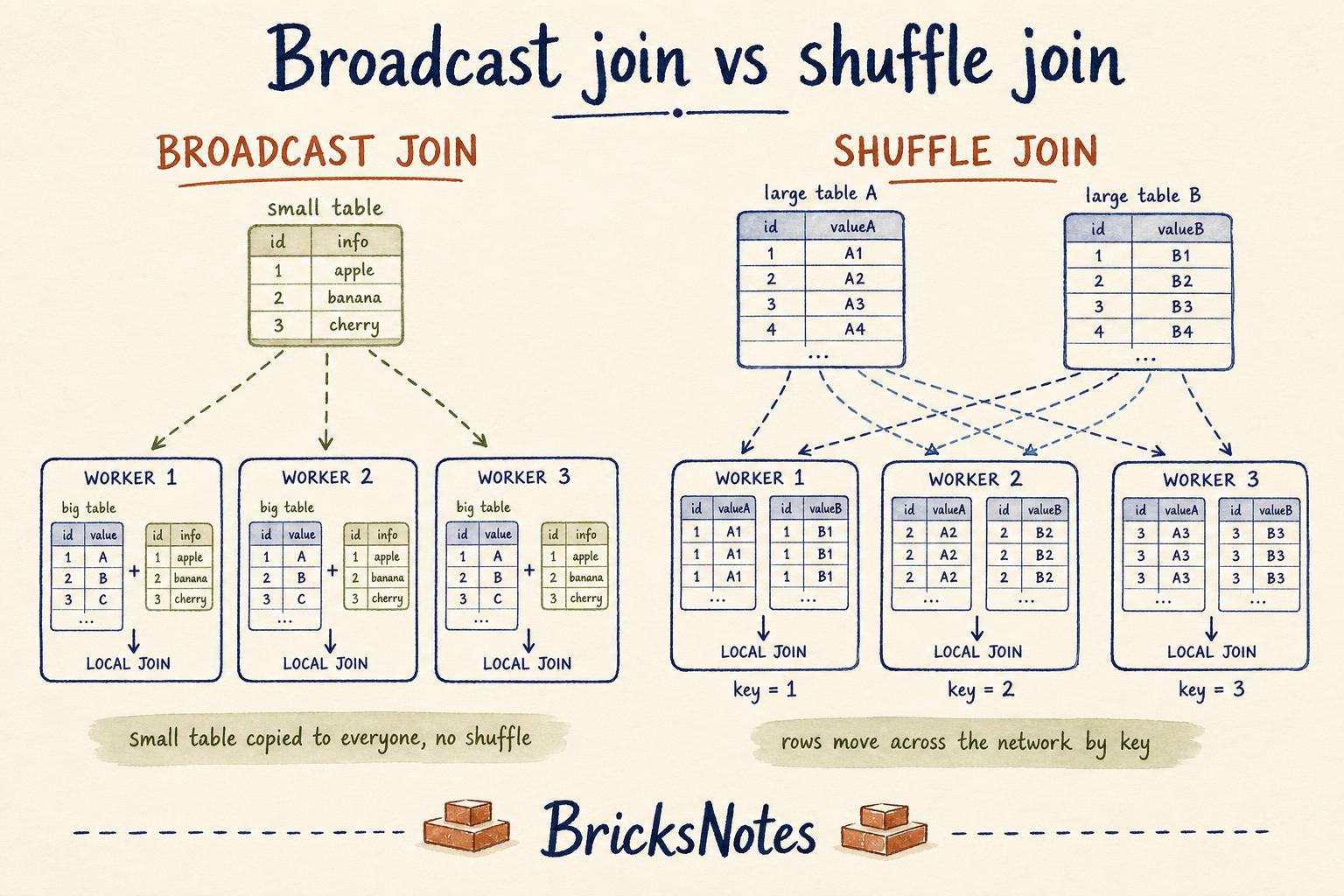
Shuffle join. Both tables get repartitioned by the join key and sent across the network, so all rows with customer_id = 42 end up on the same worker. Then each worker joins its own slice locally. This works for any size, and it costs network, disk, and time.
Broadcast join. If one side is small, Spark sends a full copy of it to every worker. Now each worker already has everything it needs, and the big table never moves at all. No shuffle. This is often ten times faster.
Same result. Very different bill.
The mental model is worth keeping: a join is not a lookup, it is a data movement plan. Once you see it that way, most performance work becomes obvious.
The rule that solves most slow joins
Ask one question before anything else. Is one side small?
A dimension table usually is. Customers, products, stores, currency codes, country lookups. A few thousand rows, maybe a few hundred megabytes at most.
If yes, broadcast it.
from pyspark.sql import functions as F

# customers is small, orders is large
enriched_orders = orders.join(
    F.broadcast(customers),
    on="customer_id",
    how="left"
)
In SQL you can say the same thing with a hint.
SELECT /*+ BROADCAST(c) */
  o.order_id,
  o.amount,
  c.region
FROM orders AS o
LEFT JOIN customers AS c
  ON o.customer_id = c.customer_id
Databricks will often choose a broadcast on its own when it knows the small side is small. The word "knows" matters. If the small side is the result of a long chain of filters and aggregations, the optimizer may only be guessing. That is when writing the hint yourself pays off.
One caution. Broadcasting sends a full copy to every worker, so it only works while the small side stays small. A dimension table that grows quietly from 200 MB to 4 GB will turn a fast job into an out-of-memory failure. Broadcast the tables you know, not the tables you hope.
We walk through both join styles with runnable examples in the Joins and Aggregations lesson, using the small practice datasets from the book so you can watch the plan change with your own eyes.
When both sides are big
Sometimes there is no small side. Orders joined to order line items. Events joined to sessions. Two fact tables, both large.
Now you accept the shuffle and try to make it as cheap as possible.
Filter before you join, not after. Every row you drop early is a row that never crosses the network.
# good: shrink first, then join
recent_orders = orders.filter(F.col("order_date") >= "2026-08-01")
result = recent_orders.join(line_items, "order_id")
Select only the columns you need. A shuffle moves whole rows. Twenty unused columns is twenty columns of network traffic per row.
Join on the same key repeatedly, not on different ones. If three joins in a row all use customer_id, Spark can reuse the partitioning and skip later shuffles. If each join uses a different key, you pay for a new shuffle every time.
Match the types. Joining an int to a string forces a cast on every row and can quietly disable some optimizations. Fix the type in the bronze layer instead, which is exactly the kind of contract discipline we described in why silent schema changes are the dangerous ones.
The join that looks fine but has one hot key
Here is the case that fools people. The plan looks reasonable, most tasks finish in seconds, and one task runs for forty minutes.
That is skew. Usually a single key holds a huge share of the rows. A guest account. A default store id. A NULL customer_id that thousands of rows share.
Adaptive Query Execution handles a lot of this for you now. It watches the actual partition sizes at runtime and splits oversized ones. It is on by default, and it is one of the best reasons to stop hand-tuning shuffle partitions.
When it is not enough, you spread the hot key yourself with salting. We covered the full technique in data skew in Databricks, explained, including how to spot the culprit key in a couple of lines of code.
Also worth checking, because it is embarrassingly common: are you joining on a column full of NULL? Every NULL fails to match, but the rows still travel. Filter them out or handle them explicitly first.
How to pick, in order
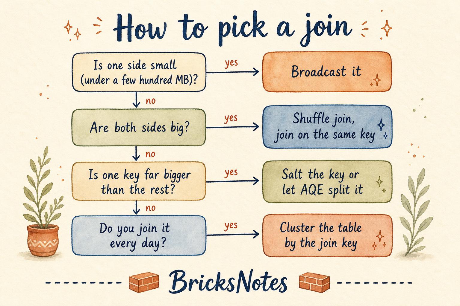
Work down the list. Stop at the first yes.
Is one side small? Broadcast it.
Are both sides big? Shuffle, and shrink both sides before the join.
Is one key far bigger than the rest? Let AQE split it, or salt it.
Do you join this table on the same key every single day? Then stop tuning the query and change the storage. Cluster the table by the join key so the files themselves are organised for it, the way we compared in Z-ORDER or liquid clustering.
How to actually see what your join is doing
You do not have to guess. Ask the plan.
enriched_orders.explain("formatted")Look for the join node. BroadcastHashJoin means no shuffle for the big side. SortMergeJoin means both sides are being repartitioned and sorted. Neither is wrong. But if you expected a broadcast and you see a sort merge join, you have learned something useful in three seconds.
Then open the Spark UI and look at the stage. If one task duration is wildly larger than the median, you have skew, not a sizing problem. Reading those numbers with confidence is a skill in itself, and it is what the Debugging and Monitoring lesson is built around.
A slow job is rarely a mystery. It is usually a plan you never looked at.
What happened to the 2 a.m. job
The customers table was 40 MB. Forty megabytes, joined to a table with 900 million rows, and Spark had planned a full shuffle of both sides because the small side arrived through a view with a filter the optimizer could not see through.
One F.broadcast(). The job went from seven hours to nine minutes.
That is the honest shape of most performance work in Databricks. Not clever code. Not a bigger cluster. Just noticing where the data is being asked to move, and asking it to move less.
Try it yourself
The fastest way to make this stick is to run both plans on the same data and compare.
Load two of the practice CSV files, join them once normally and once with a broadcast hint, and run .explain("formatted") on each. You will see the join node change. Then check the stage times.
If you want a guided version of that, the Joins and Aggregations and Partitioning and Performance lessons in BricksNotes take you through it step by step in Databricks Free Edition, with datasets small enough to run instantly and shaped badly enough to be interesting.
Start with the plan. The speed follows.